Using pandas for data analysis
Overview
Teaching: 0 min
Exercises: 0 minQuestions
What is pandas?
How do I access data in a pandas dataframe?
Objectives
Use pandas to examine and analyze data
Pandas is another Python package which is very popular for data analysis. The key feature of pandas is the dataframe. In this lesson, we will cover pandas dataframes and some basic analysis.
What is pandas?
You are already familiar with the data analyis library numpy and the numpy array. NumPy is useful when you are working with data that is all numeric. Pandas, however, is capable of handling data of lots of different types. It is designed to make working with “relational” or “labeled” data easy and intuitive. Central to the pandas package are the special data structures called pandas Series and DataFrames. Pandas dataframes are 2 dimensional and tabular, and is particularly suited to data which is heterogenous and in columns, like an SQL table or Excel spreadsheet. In fact, there are even functions which allow you to read data directly from excel spreadsheets or SQL databases (more on this later).
Pandas is built to closely work with NumPy. Many functions which work on NumPy arrays will also work on Pandas DataFrames.
To use pandas, you must first make sure it is installed, then import it. If you do not have pandas installed, install it using conda with the following command
conda install -c anaconda pandas
Next, open a new Jupyter notebook and import the module. When imported, pandas is typically abbreviated to pd
import pandas as pd
Reading data
Today, we will be working with a data set that contains information about the elements in the periodic table (2019 is the International Year of the Periodic Table!).The data is a csv (comma separated value) file from PubChem. You can download the file here.
Once you have the file downloaded and saved in your directory, we will load it into pandas. This file is a csv (comma separated value) file, so we will load it using the pd.read_csv command.
periodic_data = pd.read_csv('PubChemElements_all.csv')
Since this file is relatively simple, we do not need any additional arguments to the function. The read_csv function reads in tabular data which is comma delimited by default.
Examining the data
The variable periodic_data is now a pandas DataFrame with the information contained in the csv file. You can examine the DataFrame using the .head() method. This shows the first 5 rows stored in the DataFrame.
periodic_data.head()
| AtomicNumber | Symbol | Name | AtomicMass | CPKHexColor | ElectronConfiguration | Electronegativity | AtomicRadius | IonizationEnergy | ElectronAffinity | OxidationStates | StandardState | MeltingPoint | BoilingPoint | Density | GroupBlock | YearDiscovered | |
|---|---|---|---|---|---|---|---|---|---|---|---|---|---|---|---|---|---|
| 0 | 1 | H | Hydrogen | 1.008000 | FFFFFF | 1s1 | 2.20 | 120.0 | 13.598 | 0.754 | +1, -1 | Gas | 13.81 | 20.28 | 0.000090 | Nonmetal | 1766 |
| 1 | 2 | He | Helium | 4.002600 | D9FFFF | 1s2 | NaN | 140.0 | 24.587 | NaN | 0 | Gas | 0.95 | 4.22 | 0.000179 | Noble gas | 1868 |
| 2 | 3 | Li | Lithium | 7.000000 | CC80FF | [He]2s1 | 0.98 | 182.0 | 5.392 | 0.618 | +1 | Solid | 453.65 | 1615.00 | 0.534000 | Alkali metal | 1817 |
| 3 | 4 | Be | Beryllium | 9.012183 | C2FF00 | [He]2s2 | 1.57 | 153.0 | 9.323 | NaN | +2 | Solid | 1560.00 | 2744.00 | 1.850000 | Alkaline earth metal | 1798 |
| 4 | 5 | B | Boron | 10.810000 | FFB5B5 | [He]2s2 2p1 | 2.04 | 192.0 | 8.298 | 0.277 | +3 | Solid | 2348.00 | 4273.00 | 2.370000 | Metalloid | 1808 |
Pandas has read the data into a table. The first row of the file was used for column headers.
Previewing the end of the DataFrame
You can see the last 5 rows of the dataframe using the
.tail()command. For example, to see the last 5 rows of our DataFrame, we would typeperiodic_data.tail()
You can also see information about the DataFrame using the .info() method.
periodic_data.info()
<class 'pandas.core.frame.DataFrame'>
RangeIndex: 118 entries, 0 to 117
Data columns (total 17 columns):
AtomicNumber             118 non-null int64
Symbol                   118 non-null object
Name                     118 non-null object
AtomicMass               118 non-null float64
CPKHexColor              108 non-null object
ElectronConfiguration    118 non-null object
Electronegativity        95 non-null float64
AtomicRadius             113 non-null float64
IonizationEnergy         102 non-null float64
ElectronAffinity         57 non-null float64
OxidationStates          103 non-null object
StandardState            118 non-null object
MeltingPoint             103 non-null float64
BoilingPoint             93 non-null float64
Density                  96 non-null float64
GroupBlock               118 non-null object
YearDiscovered           118 non-null object
dtypes: float64(8), int64(1), object(8)
memory usage: 15.8+ KB
–
- First, the data type is listed. This is a pandas DataFrame. Next, it tells us that we have 118 rows (118 entries) in the DataFrame.
- There are 17 columns of data
- Next, the name of each column along with the number of entries for that column, and the data type for that column. Note that for some columns, such as
Electronegativity, there are fewer than 118 entries. This occurs because data is missing for some elements. Whenpandasread in our data file, it replaced these missing values withNaN(or ‘not a number’).
We can also see descriptive statistics easily using the .describe() command.
periodic_data.describe()
| AtomicNumber | AtomicMass | Electronegativity | AtomicRadius | IonizationEnergy | ElectronAffinity | MeltingPoint | BoilingPoint | Density | |
|---|---|---|---|---|---|---|---|---|---|
| count | 118.000000 | 118.000000 | 95.000000 | 113.000000 | 102.000000 | 57.000000 | 103.000000 | 93.000000 | 96.000000 |
| mean | 59.500000 | 146.607635 | 1.732316 | 201.902655 | 7.997255 | 1.072140 | 1273.740553 | 2536.212473 | 7.608001 |
| std | 34.207699 | 89.845304 | 0.635187 | 42.025707 | 3.339066 | 0.879163 | 888.853859 | 1588.410919 | 5.878692 |
| min | 1.000000 | 1.008000 | 0.700000 | 120.000000 | 3.894000 | 0.079000 | 0.950000 | 4.220000 | 0.000090 |
| 25% | 30.250000 | 66.480000 | 1.290000 | 180.000000 | 6.020500 | 0.470000 | 516.040000 | 1180.000000 | 2.572500 |
| 50% | 59.500000 | 142.573850 | 1.620000 | 202.000000 | 6.960000 | 0.754000 | 1191.000000 | 2792.000000 | 7.072000 |
| 75% | 88.750000 | 226.777165 | 2.170000 | 229.000000 | 8.998500 | 1.350000 | 1806.500000 | 3618.000000 | 10.275250 |
| max | 118.000000 | 294.214000 | 3.980000 | 348.000000 | 24.587000 | 3.617000 | 3823.000000 | 5869.000000 | 22.570000 |
The describe function lists the mean, max, min, standard deviation and percentiles for each column excluding NaN values.
Accessing Data
Data in pandas DataFrames are stored in rows and columns.
Accessing data using row and column numbers
Pandas DataFrames are organized using columns, which we have already discussed and index for the rows.
To access data using the row number and column number, use the .iloc method.
Data in pandas DataFrames can be accessed using slices in the same way as NumPy arrays using the iloc method.
# This will access row 35 (counting starting at 0)
periodic_data.iloc[35]
AtomicNumber                           36
Symbol                                 Kr
Name                              Krypton
AtomicMass                           83.8
CPKHexColor                        5CB8D1
ElectronConfiguration    [Ar]4s2 3d10 4p6
Electronegativity                       3
AtomicRadius                          202
IonizationEnergy                       14
ElectronAffinity                      NaN
OxidationStates                         0
StandardState                         Gas
MeltingPoint                       115.79
BoilingPoint                       119.93
Density                          0.003733
GroupBlock                      Noble gas
YearDiscovered                       1898
Name: 35, dtype: object
or, you can use slicing syntax.
periodic_data.iloc[35:45]
Like NumPy arrays, the second index is taken to be the column number.
# This selects the row 1 and column 2.
periodic_data.iloc[1, 2]
Check your understanding
Use the
ilocfunction to
Select row 5
Select rows 30 to the end.
Select column 2 through 4 and rows 50 to the end, every other row.Solution
periodic_data.iloc[5]
periodic_data.iloc[30:]
periodic_data.iloc[50::2, 2::5]
Accessing information by name
Indices in pandas can either be identified using numbers (as in the row number, similar to numpy arrays), or by name using column names and index names.
Accessing columns of data
Unless otherwise specified in the read_csv command, pandas will use the first row of the file as column names. You can use these column names to access data in a particular column.
To see all of the column names, you can type
periodic_data.columns
Index(['AtomicNumber', 'Symbol', 'Name', 'AtomicMass', 'CPKHexColor',
       'ElectronConfiguration', 'Electronegativity', 'AtomicRadius',
       'IonizationEnergy', 'ElectronAffinity', 'OxidationStates',
       'StandardState', 'MeltingPoint', 'BoilingPoint', 'Density',
       'GroupBlock', 'YearDiscovered'],
      dtype='object')
To access columns of data in pandas, you use the syntax
# Syntax for selecting pandas column
# dataframe_name['column name']
For example, to access the data in the Electronegativity column, we would use the syntax
periodic_data['Electronegativity']
0      2.20
1       NaN
2      0.98
3      1.57
4      2.04
       ...
113     NaN
114     NaN
115     NaN
116     NaN
117     NaN
Name: Electronegativity, Length: 118, dtype: float64
If you would like to select multiple columns of data, you put multiple column names in a list.
periodic_data[['Name','Electronegativity']]
    Name	    Electronegativity
0	Hydrogen	2.20
1	Helium	    NaN
2	Lithium	    0.98
3	Beryllium	1.57
4	Boron	    2.04
...	...	...
113	Flerovium	NaN
114	Moscovium	NaN
115	Livermorium	NaN
116	Tennessine	NaN
117	Oganesson	NaN
118 rows × 2 columns
Check your understanding
How would you select the columns ‘Name’, ‘AtomicMass’, and ‘StandardState’’.
Solution
To select these columns, you would put them in a list in square brackets (
[]) following the name of the DataFrame.periodic_data[['Name', 'AtomicMass', 'StandardState']]
Accessing rows and columns by name
We have already discussed column names, but what about row names? By default, the names of the rows are the same as the numbers. You may have noticed that when you are printing your dataframes, there is an extra first column of numbers going from 0 to 118. These are the row names. Unless otherwise specified in the read_csv command, the row names will default to the row number.
To access rows using the row name, use the .loc method. Currently our row names and numbers are the same, so this does not look any different than using iloc if only one index is specified.
periodic_data.loc[35]
AtomicNumber                           36
Symbol                                 Kr
Name                              Krypton
AtomicMass                           83.8
CPKHexColor                        5CB8D1
ElectronConfiguration    [Ar]4s2 3d10 4p6
Electronegativity                       3
AtomicRadius                          202
IonizationEnergy                       14
ElectronAffinity                      NaN
OxidationStates                         0
StandardState                         Gas
MeltingPoint                       115.79
BoilingPoint                       119.93
Density                          0.003733
GroupBlock                      Noble gas
YearDiscovered                       1898
Name: 35, dtype: object
However, now we can use the column name instead of the column number.
periodic_data.loc[35, 'YearDiscovered']
'1898'
Let’s see what happens when we change our index to one of our columns, so that we can use loc to access data by name. Imagine that we wanted to be able to access rows in our DataFrame using the element symbol. We will use the command set_index to do this.
periodic_data.set_index('Symbol')
This will print your new DataFrame to the screen. You should notice that now the left most column is named ‘Symbol’ and lists the symbols for each element. Let’s try accessing Kr using loc.
periodic_data.loc['Kr']
KeyError: 'Kr'
It didn’t work! Why? Examine periodic_data again. The index is the same as before. This is because the .set_index method returns a new copy of the dataframe. If we wish to have later access to this copy, we have two options. We can capture the value in a variable (as in periodic_data_index = periodic_data.set_index('Symbol')).
periodic_data_symbols = periodic_data.set_index('Symbol')
periodic_data_symbols.loc['Kr']
AtomicNumber                           36
Name                              Krypton
AtomicMass                           83.8
CPKHexColor                        5CB8D1
ElectronConfiguration    [Ar]4s2 3d10 4p6
Electronegativity                       3
AtomicRadius                          202
IonizationEnergy                       14
ElectronAffinity                      NaN
OxidationStates                         0
StandardState                         Gas
MeltingPoint                       115.79
BoilingPoint                       119.93
Density                          0.003733
GroupBlock                      Noble gas
YearDiscovered                       1898
Name: Kr, dtype: object
This lists all the information for the entry. Note the bottom, where it says Name: Kr, dtype: object. Kr is what we used for the index.
You can use row, column indexing with both the loc and iloc command. For example, to get the boiling point of Kr, you could use
periodic_data_symbols.loc['Kr', 'BoilingPoint']
119.93
Note that this is the same order as before - row, followed by column.
The same information could have been accessed (though less conveniently) using iloc. This would require you to know the numerical position of the ‘BoilingPoint’ column.
periodic_data_symbols.iloc[35, 12]
119.93
or, you could have combined ways to access data.
periodic_data_symbols['BoilingPoint'].iloc[35]
119.93
Check your understanding
How would you access each of the following:
The electron configuration of Boron.
The atomic radius of the element on row 115.
The value in cell (50, 5).Solution
periodic_data_symbols.loc['B', 'ElectronConfiguration']
periodic_data_symbols['AtomicRadius'].iloc[115]
periodic_data_symbols.iloc[50,5]
Another option for setting the index
Instead of making a new variable (
periodic_data_symbols), we might have chose to overwrite our existing dataframe. In pandas, you can do that by adding an additional argument to yourset_indexfunction.We can use the keyword argument
inplace=True. When we use this argument, pandas will overwrite the original DataFrame. Always look for this argument in pandas functions.periodic_data.set_index('Symbol', inplace=True)If you wanted to change your index back to numbers, you would use the command
reset_indexperiodic_data.reset_index(inplace=True)This is a very important command. If you set another index without resetting the index, the
Symbolcolumn will be lost. This comman reverts it back to a column.
Broadcating and such
Like NumPy arrays, pandas also takes advantage of broadcasting. You can add scalars or vectors to data easily.
We could calculate the melting point in celsius
periodic_data_symbols['MeltingPoint'] - 273.15
Symbol
H     -259.34
He    -272.20
Li     180.50
Be    1286.85
B     2074.85
       ...
Fl        NaN
Mc        NaN
Lv        NaN
Ts        NaN
Og        NaN
If you would like to capture this in a new DataFrame column, you can do so easily by putting the new column name in square brackets following the DataFrame name.
periodic_data_symbols['MeltingPointC'] = periodic_data_symbols['MeltingPoint'] - 273.15
Check your understanding
Make a new column in your DataFrame called ‘BoilingPointC’ where you have converted the boiling points from Kelvin to Celsius.
Solution
This is very similar to how you created MeltingPointC.
periodic_data_symbols['BoilingPointC'] = periodic_data_symbols['BoilingPoint'] - 273.15
But what if we wanted to use a function instead of a scalar? Imagine you had written a function to convert temperatures in Kelvin to Fahrenheit.
def kelvin_to_fahrenheit(kelvin_temp):
    fahrenheit = (kelvin_temp - 273.15) * 9/5 +32
    return fahrenheit
If you wanted to apply this function to every row, your first instinct might be to write a for loop. This would work, but pandas has a built in method called apply to easily allow you to do this.
When you call the apply method, you give it a function name which you would like to apply to every element of whatever you are using it on.
# Calculate the boiling point in fahrenheit
periodic_data_symbols['BoilingPoint'].apply(kelvin_to_fahrenheit)
Symbol
H     -423.166
He    -452.074
Li    2447.330
Be    4479.530
B     7231.730
        ...
Fl         NaN
Mc         NaN
Lv         NaN
Ts         NaN
Og         NaN
Name: BoilingPoint, Length: 118, dtype: float64
To save it as a new column
periodic_data['BoilingPointF'] = periodic_data['BoilingPoint'].apply(kelvin_to_fahrenheit)
Saving your new Dataframe
If you wanted to save your data as a csv, you could do it using the command to_csv
periodic_data_symbols.to_csv('periodic_data_processed.csv')
Filtering and sorting your DataFrame
Use .query to filter data
You can use the function .query to query your data. You type a logical expression in a string inside of the function.
For example, to find all of the elements with a melting point greater than 298,
periodic_data.query('MeltingPoint > 298')
You can combine several statements.
periodic_data.query('MeltingPoint > 298 and BoilingPoint < 500')
You can even use this synatx to compare two columns to one another.
periodic_data.query('MeltingPoint > BoilingPoint')
Use .sort_values to sort data
To sort data, you can use the sort_values function.
periodic_data.sort_values(by='MeltingPoint')
This will sort the rows (axis=0) by the values in the ‘MeltingPoint’ column. If you are familiar with Excel, this is similar to how spreadsheets are sorted if you sort based on one of the columns. This sort will return a DataFrame where elements with the lowest melting point are listed first.
It is also possible to columns based on values in a row. However, they all have to be the same type (numeric or string).
For example,
numeric_data = periodic_data[['AtomicNumber', 'BoilingPoint', 'AtomicMass', 'MeltingPoint']].copy()

numeric_data.head()
numeric_data.sort_values(by='Au', axis=1)
Note how the column orders change.
Use .groupby to group data
You can also group values in a DataFrame using the groupby function.
grouped_data = periodic_data.groupby(by='StandardState')
Here, we are grouping the DataFrame based on values in the column ‘ExpectedState’.
We can see the groups which have been created by using .groups
grouped_data.groups
{'Expected to be a Gas': Int64Index([117], dtype='int64'),
 'Expected to be a Solid': Int64Index([109, 110, 111, 112, 113, 114, 115, 116], dtype='int64'),
 'Gas': Int64Index([0, 1, 6, 7, 8, 9, 16, 17, 35, 53, 85], dtype='int64'),
 'Liquid': Int64Index([34, 79], dtype='int64'),
 'Solid': Int64Index([  2,   3,   4,   5,  10,  11,  12,  13,  14,  15,  18,  19,  20,
              21,  22,  23,  24,  25,  26,  27,  28,  29,  30,  31,  32,  33,
              36,  37,  38,  39,  40,  41,  42,  43,  44,  45,  46,  47,  48,
              49,  50,  51,  52,  54,  55,  56,  57,  58,  59,  60,  61,  62,
              63,  64,  65,  66,  67,  68,  69,  70,  71,  72,  73,  74,  75,
              76,  77,  78,  80,  81,  82,  83,  84,  86,  87,  88,  89,  90,
              91,  92,  93,  94,  95,  96,  97,  98,  99, 100, 101, 102, 103,
             104, 105, 106, 107, 108],
            dtype='int64')}
We can then retrieve any group by name. For example, to get the data associated with gases,
grouped_data.get_group('Gas')
This will return a pandas DataFrame where all of the elements returned have the expected state of Gas.
Grouping is particularly useful for calculating statistics about data that fits a particular criteria.
for group, data in grouped_data:
    print(group, data['BoilingPoint'].mean(), data['BoilingPoint'].std())
Expected to be a Gas nan nan
Expected to be a Solid nan nan
Gas 102.45272727272727 76.27220858096467
Liquid 480.91499999999996 210.6683233189081
Solid 2922.236875 1361.7433032823824
Built-in Plotting
Looking at our data above, we notice very high standard deviations for some of the groups. One way we might examine this visually by looking at a histogram plot.
Pandas DataFrames have several built-in plotting functions, one of which is .hist. If we call this function on just a DataFrame, it will make a histogram for each column of data.
In our case, we are interested in the histogram for each group we have created.
We could make histograms for each of our groups by adding this command into our for loop.
for group, data in grouped_data:
    print(group, data['BoilingPoint'].mean(), data['BoilingPoint'].std())
    data.hist(column='BoilingPoint')
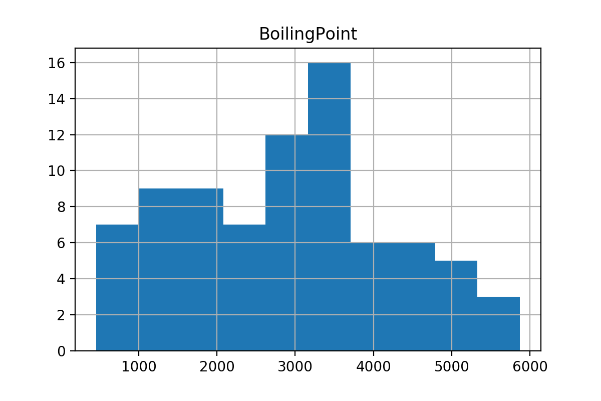
You should see a histogram for each group after executing this cell. The histogram for ‘Solid’ is shown below.
Exercise
Modify your
forloop so that each graph has a title which is the group name. Save each image as a png with resolution 200 dpi with the file namegroup_name_bp_hist.png.Solution
for group, data in grouped_data:
   print(group, data['BoilingPoint'].mean(), data['BoilingPoint'].std())
   data.hist(column='BoilingPoint')
   plt.title(group)
   plt.savefig(F'{group}_bp_hist.png', dpi=200)
You could have also gotten all of the histograms in the same figure
periodic_data.hist(column='BoilingPoint', by='StandardState')
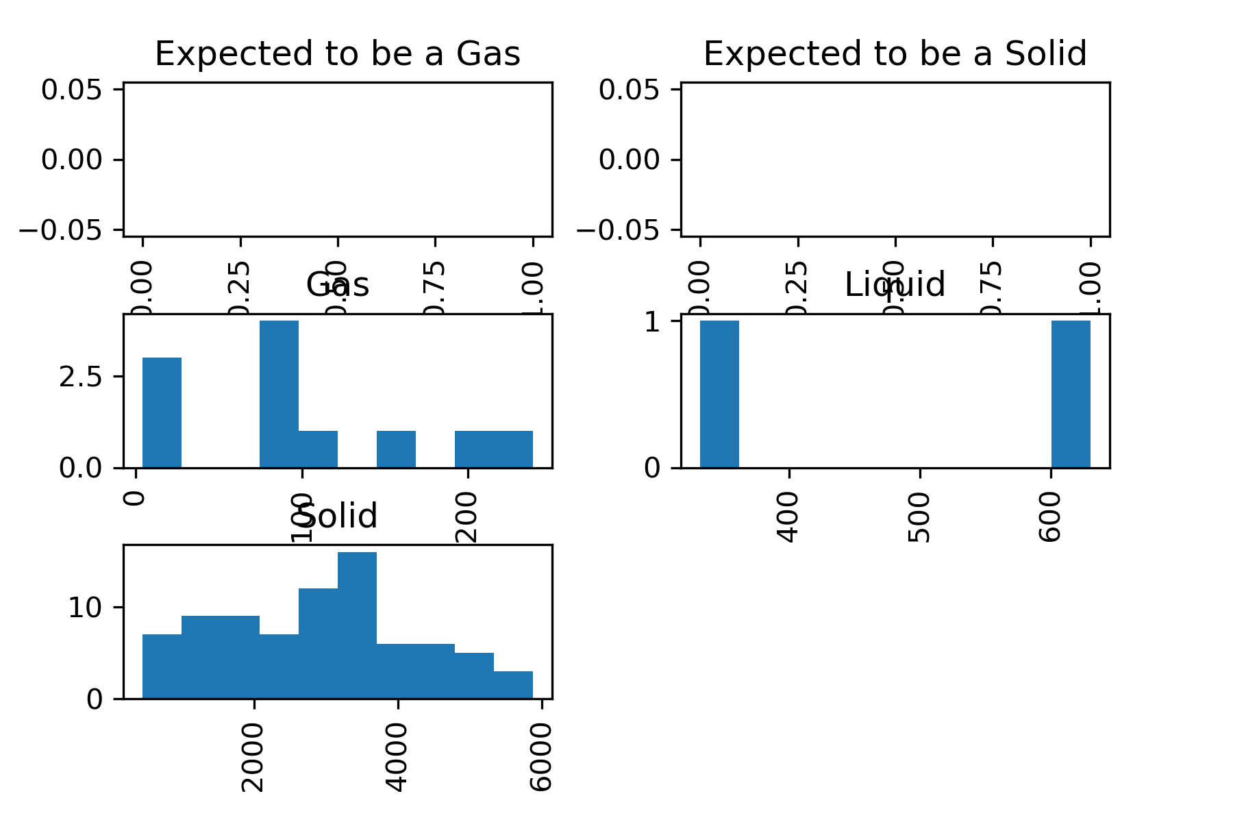
However, you can see that this is a little hard to read. It would be possible to make this plot more readable, but we will not cover that in this lesson.
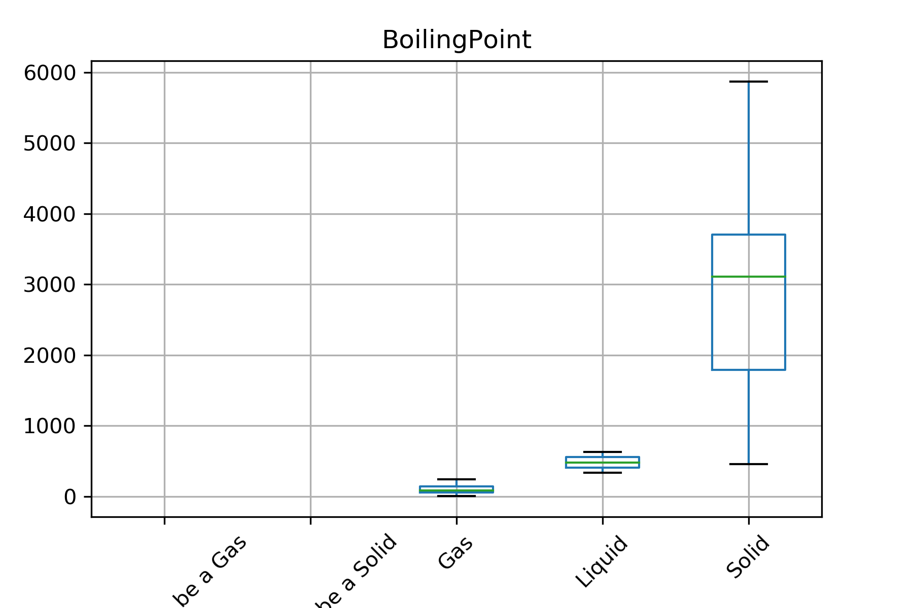
Another plotting option you might have chosen was a boxplot
periodic_data.boxplot(column='BoilingPoint', by='StandardState', rot=90)

plt.suptitle("")
These are just a few examples of visualizations you can do on pandas DataFrames. You can read more in the pandas documentation.
Key Points
Pandas stores data in a structure called a dataframe
Pandas can read data that has lots of different data types.
You can easily get statistics from a dataframe by using methods like df.describe()